EU Forest, Visualizing More Than 500,000 Trees Using Google Maps and Deck.gl
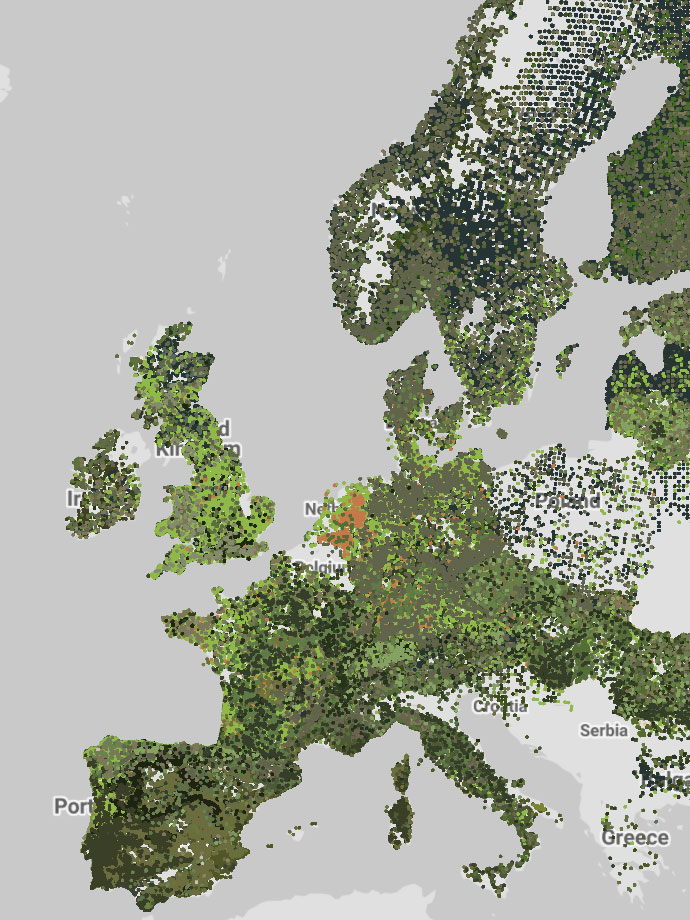
Sometimes we encounter projects that push the limits of Google Maps. One of the biggest challenges developers face when using this tool is the need to display thousands—or even hundreds of thousands—of points on a custom map. Is this even possible?
Google Maps and its API have evolved significantly over the past few years. They now offer concepts
like Custom Overlays, which extend the inherent capabilities of the platform. This evolution also creates a flexible
environment for integrating projects like deck.gl seamlessly.
In this article, I share my experience representing 588,983 trees on a standard Google Maps implementation. I encourage you to grab your favorite drink and join me on this journey. (☕|🥤|🍺|🍷)
Table of Contents
- The Inspiration
- Selecting the Problem
- Coordinate Systems: More Than Latitude and Longitude
- Getting Trees Colors
- And, What is deck.gl?
- Integrating deck.gl and Google Maps
- Conclusion
- References and Links
The Inspiration
Last year, I had the opportunity to see Alex Muramoto give a talk titled “Awesome Web Data Viz with Google Maps Platform and deck.gl.” If you didn’t get a chance to attend one of the many DevFest events where Alex presented, you can watch the talk on YouTube using this link: https://bit.ly/alexsgmapdeckgl.
During the talk, Alex guided us through various examples that extend the capabilities of Google Maps using deck.gl. He demonstrated how to create more than just a simple marker—you can add multiple points, arcs, and even create real-time visualizations in specific map regions. This inspired me to experiment with these two technologies.
Selecting the Problem
While researching online, I found a variety of complete datasets from websites such as the Paris Open Data Site and the European Data Portal. I also came across several papers on geospatial visualization. One paper that caught my eye was “EU-Forest, a High-Resolution Tree Occurrence Dataset for Europe”1. The paper details the methodology used to curate information on European tree species to produce a unique dataset that is well distributed across countries. One of its best features is that the dataset is open and provides valuable details—such as coordinates, species, and visualization examples—that serve as useful guidelines.
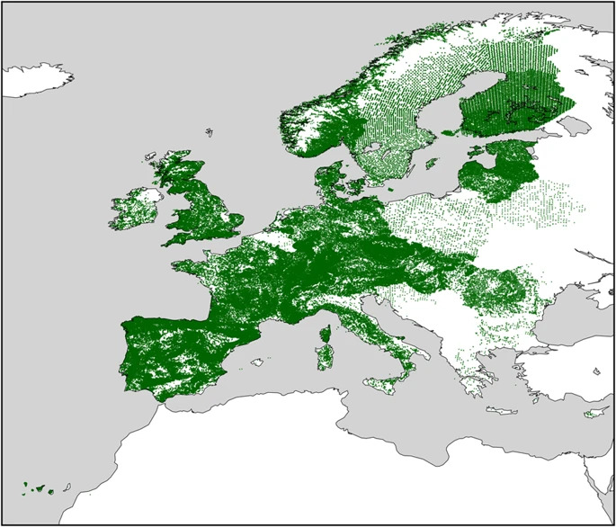
Spatial distribution of all occurrences in EU forest.
With all that in place, it was exciting to reproduce the experiment using Google Maps and deck.gl.
Coordinate Systems: More Than Latitude and Longitude
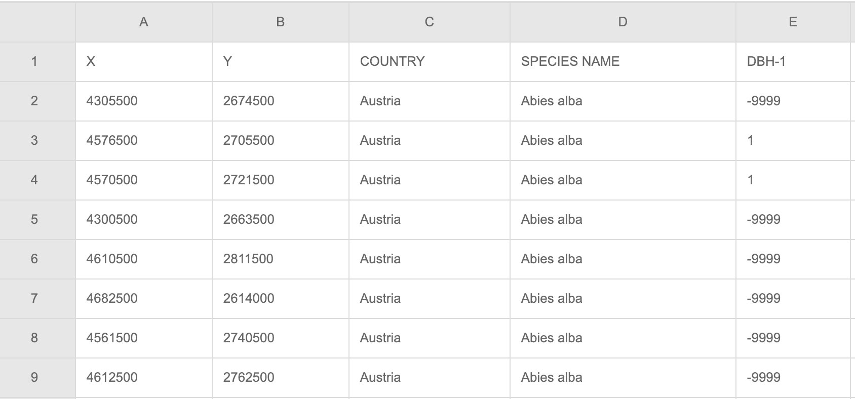
On the publication’s webpage, you will find various documents. The one we will use as a
reference2 for our visualization is curated based
on tree species.
This file is in CSV format and, as indicated in
the metadata file, the X and Y
coordinates use the ETRS89-LAEA reference system… 🤨. And now, the fun begins!
Typically, the libraries or map services we integrate into our code instruct us to reference positions using latitude and longitude. Therefore, the first challenge I faced when processing the dataset was understanding and transforming the coordinate values from the file into a format that makes sense for deck.gl or Google Maps.
It’s time to seek help from Google Search! I discovered that ETRS89-LAEA is equivalent to EPSG:3035… With this in
mind, we can now tackle this initial challenge.
EPSG
EPSG stands for “European Petroleum Survey Group.” This group produced various datasets aimed at providing reliable spatial references that can be applied globally, regionally, nationally, and locally. In theory, one of these datasets corresponds to the coordinate system that uses latitude and longitude.
One of the most useful resources I found—allowing you to work with these references easily—is epsg.io. On this site, you can transform coordinate values between different systems.
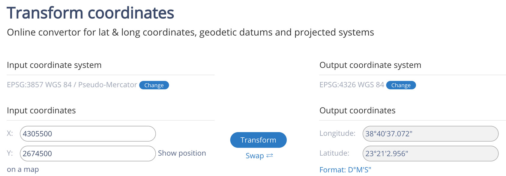
After a quick inspection of the code, I realized that they were using a library called proj4JS – bingo! This is exactly
what I needed to start the data conversion. 😁 Thanks to them, I obtained a full list of all EPSG codes, which allowed me
to convert the dataset to the traditional coordinate system, EPSG:4326.
proj4JS
proj4JS is an open-source project inspired by libraries such as PROJ. This library enables conversion between coordinate systems—a very specialized niche in software development. Sometimes the documentation is insufficient or hard to understand regarding the underlying calculations.
You can install proj4 via npm or yarn to start using it. According to the documentation, the function usage is as
follows:
  proj4(fromProjection[, toProjection, coordinates
])
The required values reference projections3. A projection is the mathematical operation needed to convert coordinates between systems. While the PROJ project explains these calculations in detail, for now we will focus on the values. Understanding how these formulas are formed could be the subject of another post.
To define the projection for EPSG:3035, you need to write the following array:
[
  'EPSG:3035',
  '+proj=laea +lat_0=52 +lon_0=10 +x_0=4321000 +y_0=3210000 +ellps=GRS80 +towgs84=0,0,0,0,0,0,0 +units=m +no_defs ',
];
As mentioned, the projection value can be complex at first, and mistakes often occur due to typos. That’s why I created a repository with a list of values that lets you obtain the projection string for any EPSG code using an index. The list contains 6137 entries for conversion. You can read the full list and see the names in the project’s README file. To use it with proj4, write the following code:
const proj4 = require("proj4")
const proj4list = require("./list.min");
proj4.defs([
  proj4list["EPSG:3035"],
  proj4list["EPSG:4326"]
);
proj4("EPSG:3035", "EPSG:4326", [4305500, 2674500]);
Now we have a way to convert the original X and Y values from the dataset into latitude and longitude! Our script to convert the CSV file to JSON will follow this logic:
- 📃 Read each row in the CSV document.
- 🗺 Convert X and Y to latitude and longitude.
- 🌲 Replace the tree species with a number that can be mapped to manage the colors.
The content of our dataset will look like this:
[
  {
    "specie": 70,
    "lat": 35.01966518543305,
    "lng": 32.6269824790667
  },
  ...
]
If you would like access to the final dataset, you can find the information classified by country in the following repository: Datasets: EU-Forest
Getting Trees Colors
The visualization we aim to create could work well using just the tree positions, resulting in an outcome similar to what’s presented in the paper. However, as users who constantly consume information, it’s important to represent the data accurately and create an engaging, understandable experience.
With that in mind, let’s start working on this part. The main idea is to fetch a couple of images from Google Search Images, merge them, and extract the dominant color.
To help with this, I found a Node.js library that uses Puppeteer called images-scraper, which returns an array of image URLs based on a query.
const scraper = require('images-scraper');

const google = new scraper({puppeteer: {headless: true}});

function searchAndAnalize(term, limit) {
  /*
    results [
      {
        url: 'https://...',
        source: 'https://...',
        description: '...'
      },
      ...
    ]
  */
  return new Promise(async (resolve, reject) => {
    const results = await google.scrape(term, limit);
  });
}
For each element in the array, we will download the file. We need to write a function that saves the files to a directory and simultaneously stores the file paths in another array for later use. The download function is as follows:
const fs = require('fs');
const request = require('request');

async function downloadImage(url) {
  try {
    return new Promise((resolve, reject) => {
      request.head(url, function (error, res, body) {
        if (error) {
          reject(error);
        }
        let extension =
          res.headers['content-type'] === 'image/jpeg' ? 'jpg' : 'png';
        let file_name = `${collectionPath}/${new Date().getTime()}.${extension}`;
        request(url)
          .pipe(fs.createWriteStream(file_name))
          .on('close', () => {
            resolve(file_name);
          });
      });
    });
  } catch (error) {
    console.log('error in', url);
  }
}
Now that we have the downloadImage function, we can retrieve the images and merge them
using merge-img. Since we don’t know the image
dimensions, we’ll save them as PNGs for better color analysis.
function searchAndAnalize(term, limit) {
  return new Promise(async (resolve, reject) => {
    const results = await google.scrape(term, limit);

    let images = await Promise.all(
      results.map(async (result) => {
        return await downloadImage(result.url);
      })
    );

    let img = await mergeImg(images);
    const output = `${collectionPath}/result_${new Date().getTime()}.png`;

    img.write(`${output}`, async () => {
      // HERE WLL BE THE IMAGE ANALYSIS
    });
  });
}
The resulting image will look like this:
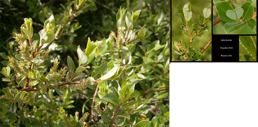
Now that we have an image to process, we will use Color Thief, a popular library for extracting the dominant color. The only parameter needed is the merged image.
img.write(`${output}`, async () => {
  resolve(await colorThief.getColor(output));
});
You can find the full code in the repository I created—access it via this link.
If you follow the installation instructions, you’ll be able to run the following command in your terminal:
node example.js palette "Batman" 10The main colors produced by this script can be found in the following file. These colors correspond to the 242 tree species processed.
And, What is deck.gl?
deck.gl is an open-source tool that is changing the way we visualize map data as developers, ultimately impacting our product customers. Created by the Uber Visualization team, it leverages WebGL2 to make better use of our hardware, allowing us to explore and visualize large amounts of data using superimposed layers in the browser. It also gives developers the ability to customize, update, or remove each layer as needed.
First Steps Using deck.gl
Alright! Now that we understand deck.gl uses layers, it’s time to put them to work and visualize something.
One characteristic I like about deck.gl is its independence from any particular map system. You can use it with technologies like Google Maps, Mapbox, or ArcGIS—or even without any map framework.
For a first introduction to deck.gl, we will use two datasets provided by geojson.xyz:
deck.gl can be used in different ways. One approach that is helpful for beginners is to directly load the script into your HTML:
html Copy
<script
  type="text/javascript"
  src="https://unpkg.com/deck.gl@latest/dist.min.js"
></script>
When adding JavaScript without webpack or a module bundler, assign the methods you need to variables or constants:
const {DeckGL, GeoJsonLayer, ArcLayer} = deck;We will also initialize three constants: two for managing the datasets and one for the central point corresponding to Mexico City Airport.
const COUNTRIES =
  'https://d2ad6b4ur7yvpq.cloudfront.net/naturalearth-3.3.0/ne_50m_admin_0_scale_rank.geojson';
const AIR_PORTS =
  'https://d2ad6b4ur7yvpq.cloudfront.net/naturalearth-3.3.0/ne_10m_airports.geojson';

const INITIAL_VIEW_STATE = {
  latitude: 19.43,
  longitude: -99.08,
  zoom: 4,
  bearing: 0,
  pitch: 30,
};
To start deck.gl, create a new instance of the main class, providing an initial state and an array of layers to display:
new DeckGL({
  initialViewState: INITIAL_VIEW_STATE,
  controller: true,
  layers: [
    // ... HERE WILL BE THE DATA LAYERS
  ],
});
Since our datasets are already in JSON format, we can use GeoJsonLayer to quickly create them. In this case, we’ll
start with the country layer:
...
layers : [
  new GeoJsonLayer({
    id: 'country-layer',    //Layer Id
    data: COUNTRIES,        //Dataset
    stroked: true,          //Stroke or Border
    filled: true,           //Fill
    lineWidthMinPixels: 1,  //Pixel Width
    opacity: 0.4,           //Opacity
    getLineColor: [154, 154, 154],  //RGB color for stroke
    getFillColor: [242, 242, 242]   //RGB color for fill
  }),
]
...
On screen, the result will look like this:
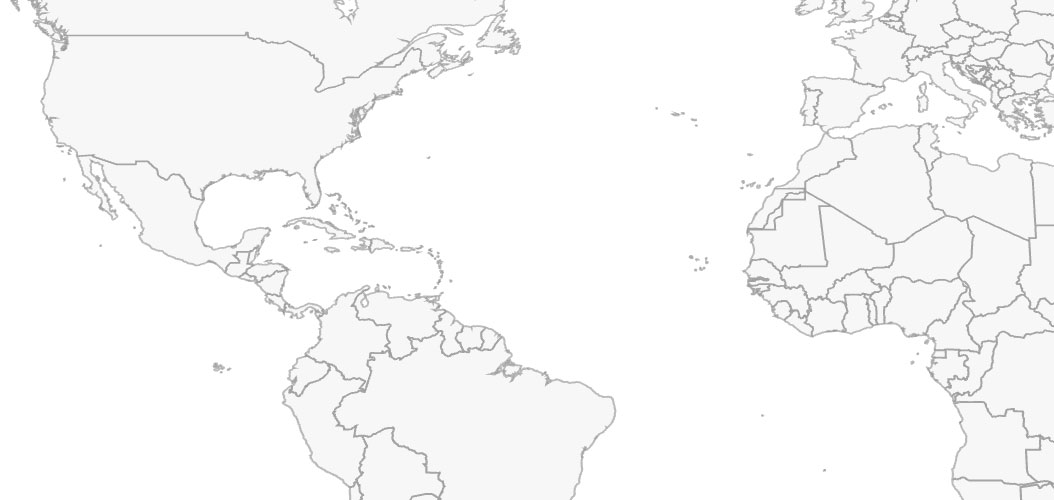
deck.gl's ability to manage layers allows us to create our own maps.
Next, we add a layer corresponding to existing airports:
...
layers : [
  ...,
  new GeoJsonLayer({
    id: 'airports',
    data: AIR_PORTS,
    filled: true,
    pointRadiusMinPixels: 2,
    pointRadiusScale: 2000,
    getRadius: f => 11 - f.properties.scalerank,
    getFillColor: [21, 192, 25],
    pickable: true,
    autoHighlight: true,
    onClick: info =>
      info.object && alert(`${info.object.properties.name}`)
  })
]
...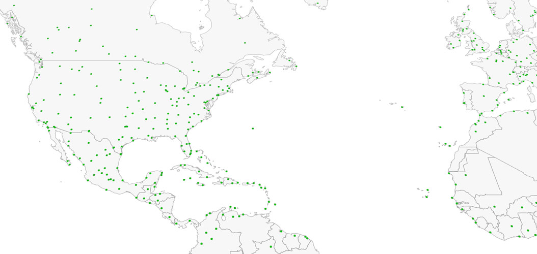
Now we have two overlays: one corresponding to the map and the other to airports.
Now we will add a new layer to display connectivity using ArcLayer. The idea is to have a single point as the origin,
from which arcs will be drawn to represent airport connections.
new ArcLayer({
  id: 'arcs',
  data: AIR_PORTS,
  dataTransform: (d) => d.features.filter((f) => true),
  getSourcePosition: (f) => [-99.08, 19.43],
  getTargetPosition: (f) => f.geometry.coordinates,
  getSourceColor: [238, 157, 30],
  getTargetColor: [21, 192, 25],
  getWidth: 1,
});
The result of these three layers is as follows:
With the dataTransform property, we can also modify how the data behaves. For example, suppose we need to display only
the connections between Mexico and the airports located within a specific longitude range, as shown in the image below:
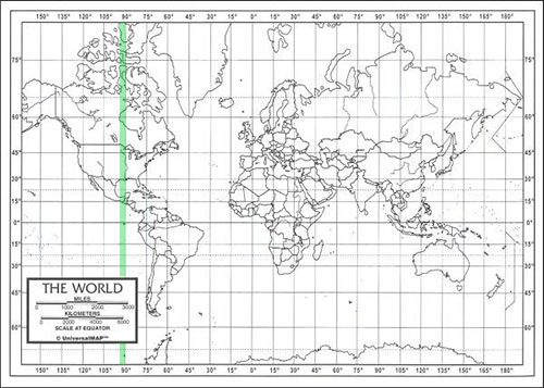
Limit between longitude: 90 and 93.
To do this, modify the attribute as follows:
const MAX = -93, MIN = -90;
...
new ArcLayer({
  ...
    dataTransform
:
d => d.features.filter(f => f.geometry.coordinates[0] < MIN && f.geometry.coordinates[0] > MAX),
...
})
...Integrating deck.gl and Google Maps
As one of the most popular mapping systems, Google Maps can be used together with deck.gl for layer management. By reading the source code, you can see that deck.gl uses Custom Overlays to achieve this integration.
...
export default class GoogleMapsOverlay {
  constructor(props) {
    this.props = {};
    this._map = null;

    const overlay = new google.maps.OverlayView();
    overlay.onAdd = this._onAdd.bind(this);
  ...
Understanding Custom Overlays
We can define Custom Overlays4 as objects that are placed on the map and
linked to specific coordinates (latitude and longitude). One of their main features is that they move when you zoom or
drag the map.
Using Custom Overlays generally involves five steps:
1.- Set the prototype
Set your custom overlay object’s prototype to a new instance of google.maps.OverlayView():
USGSOverlay.prototype = new google.maps.OverlayView();2.- Create a constructor
Create a constructor for your custom overlay and initialize any parameters:
function USGSOverlay(bounds, image, map) {
  this.bounds_ = bounds;
  this.image_ = image;
  this.map_ = map;
  this.div_ = null;
  this.setMap(map);
}
3.- Implement onAdd()
Implement an onAdd() method to attach the overlay to the map:
USGSOverlay.prototype.onAdd = function () {
  var div = document.createElement('div');
  div.style.borderStyle = 'none';
  div.style.borderWidth = '0px';
  div.style.position = 'absolute';

  var img = document.createElement('img');
  img.src = this.image_;
  img.style.width = '100%';
  img.style.height = '100%';
  img.style.position = 'absolute';
  div.appendChild(img);

  this.div_ = div;

  var panes = this.getPanes();
  panes.overlayLayer.appendChild(div);
};
4.-Implement draw()
Implement a draw() method to handle the overlay’s visual display:
USGSOverlay.prototype.draw = function () {
  var overlayProjection = this.getProjection();
  var sw = overlayProjection.fromLatLngToDivPixel(this.bounds_.getSouthWest());
  var ne = overlayProjection.fromLatLngToDivPixel(this.bounds_.getNorthEast());

  var div = this.div_;
  div.style.left = sw.x + 'px';
  div.style.top = ne.y + 'px';
  div.style.width = ne.x - sw.x + 'px';
  div.style.height = sw.y - ne.y + 'px';
};
5.-Implement onRemove()
Finally, implement an onRemove() method:
USGSOverlay.prototype.onRemove = function () {
  this.div_.parentNode.removeChild(this.div_);
  this.div_ = null;
};
Once you’ve implemented your Custom Overlay, you can invoke it within the function that initializes your map. In your
method, define the area that the image will cover using the LatLngBounds method, which takes two parameters: the
southwest and northeast coordinates. This means you first specify the bottom-left coordinate, followed by the top-right
coordinate.
function initMap() {
  //Nuestro mapa principal
  var map = new google.maps.Map(document.getElementById('map'), {
    zoom: 11,
    center: {lat: 19.487711, lng: -99.008554},
  });
  //Indicamos el área que ocupará la imagen
  var bounds = new google.maps.LatLngBounds(
    //Suroeste o inferior izquierdo
    new google.maps.LatLng(19.389876, -99.1009),
    //Noreste o superior derecho
    new google.maps.LatLng(19.599925, -98.858176)
  );
  //Imagen que agregaremos al mapa
  var srcImage = './map.png';
  //Nuestro overlay recive el área, la imagen y el mapa
  overlay = new USGSOverlay(bounds, srcImage, map);
}
In the following example, you can see the result of superimposing an image corresponding to the area of Texcoco Lake5 in Mexico City.
Google Maps Overlay and Our Trees Dataset
Alright! The time has come to apply everything we’ve learned. We already have our curated dataset of tree species and the dominant color for each species, and we now have a better understanding of how deck.gl and Custom Overlays work.
As mentioned, deck.gl provides its own method for using Custom Overlays called GoogleMapsOverlay. With it, we can
save a lot of work and time.
import { colors } from './colors'; //Tree colors

async function init() {
  await loadScript();
  const GMAP = new google.maps.Map(MAP, MAP_PROPS);

  const deckGL_overlay = new GoogleMapsOverlay();
  //Here we indicate the map that we want to use
  deckGL_overlay.setMap(GMAP);
  //Adding the layers as Array,
  deckGL_overlay.setProps({layers: [await getLayer()]});
}
As you can see in the implementation, we pass the layers as an array via the properties of the GoogleMapsOverlay
instance.
Now, we request the tree positions that were processed previously. We will implement a function named getLayer that
retrieves the data directly from the JSON file. We also assign a color to each tree based on its species index.
async function getLayer(layer = 'all') {
  //Realizamos la petición de información
  let request = await fetch(
    `https://dataset-euforest.storage.googleapis.com/country_${layer}.json`
  );
  let data = await request.json();

  return await new ScatterplotLayer({
    id: 'scatterplot-layer',
    data: data, //Esta es la inforamción de los árboles
    opacity: 1,
    stroked: false,
    filled: true,
    radiusScale: 20,
    radiusMinPixels: 1,
    radiusMaxPixels: 100,
    lineWidthMinPixels: 1,
    //Obtenemos la latitu y la longitud
    getPosition: (d) => [d.lng, d.lat],
    getRadius: (d) => 50,
    //A través del índice de la especie, retornamos el color
    getFillColor: (d) => colors[d.specie],
    getLineColor: (d) => [30, 30, 30],
  });
}
The result can be seen in the following iframe or by visiting the URL: https://eu-forest.mapsviz.com.
If you’d like, you can also visit the repository containing the full code to see how the website was built.
Conclusion
There is no doubt that the combination of deck.gl and Google Maps allows us to generate data visualizations in a very simple way—with relatively little computing power. Today, we have tools that enable us to perform geospatial analysis in entirely new ways and at a relatively low cost.
Although some tasks are already solved by specialized software, we can offer a different perspective and “democratize” data visualization thanks to web technologies. In an era when information constantly flows from various sources, helping others understand its magnitude is one of our responsibilities as Software Engineers.
For me, this experiment was a lot of fun. I learned about different methods for measuring and representing our location—from local details to global perspectives. I hope this article serves as a first step to inspire you, feed your curiosity, or act as a reference for creating an interesting new visualization.
References and links
2.- Mauri, A., Strona, G., & San-Miguel-Ayanz, J. Figshare https://dx.doi.org/10.6084/m9.figshare.c.3288407 (2016). 4.- Custom Overlays Google Maps Documentation5.- All Things living, all things dead - Cartografías del Lago de Texcoco